How to read a table correctly when the titles of lines and columns are no longer visible? To avoid being lost in anonymous cells, use the Figure Futtals: the headers will remain displayed.

How to read a table correctly when the titles of lines and columns are no longer visible? To avoid being lost in anonymous cells, use the Figure Futtals: the headers will remain displayed.

What is this or that value in the middle of a long table of figures that scrolls on the screen? Difficult to say if the titles of columns and lines disappear during scrolling! Everything becomes clear if we freeze the line of titles at the top of the table, and the first column of titles on the left: only the data on the table pass, the headers remain visible, and we always know where we are.

Excel for a long time has a special function to “fix” the lines and columns. But her name is not very explicit: her name is Freeze shutters. You will find it in all versions of Excel for Windows and Mac, as well as in Excel for the web accessible for free in your Internet browser.

Whether you want to keep lines or columns always visible on the screen, you will have to select the cells concerned in some cases before launching the function. Demonstration.

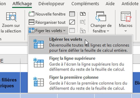
• Go to the tab Display and click on the icon Shut down. A small menu takes place which gives you access to three options: Shut down (which becomes Release the shutters When the function is activated), Upon the upper line And Freeze.

• If you check Upon the upper linethere line 1 will always remain visible when you scroll the sheet down. Which will of course only be useful if you have registered your column headers in this line 1.
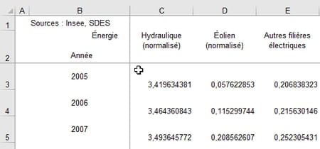
• On the example below, our headers not appearing in line 1 but in line 2the option is not useful, it is therefore necessary to proceed otherwise …

• To freeze for example the first two lines of the table: before launching the command Shut downclick on the left of the window on the line 3 To select it (you could also just select the cell A3). Now click on the icon Shut downthen below on Shut down. All lines above of the line 3 (so the lines 1 and 2) will now be displayed if you move down the table. On our example, we keep the headers on the screen Energy.

• To freeze the first five lines, it would therefore be necessary to select the line 6 or the cell A6. We would be tempted to select the lines 1 to 5 Before launching the command Shut down. Alas, it does not work! You must select a single line, that located just below the lines that must remain displayed on the screen.

• Note that once you have frozen the shutters, the first option of the small drop -down menu is renowned and is called Release the shutters. Which, you can imagine, allows you to cancel the effects.

• Below, we have rid our table of its shaping and even deleted the grid of the cells to show you a detail: Excel traces a fine vertical and/or horizontal black line to help you locate the frozen lines or columns on the screen. We see here that the lines 1 and 2 and columns A and B are frozen. The features will obviously not be visible to printing.

The principle is exactly the same as for the lines. If you plan to freeze other columns than the first, you will have to make your selection before launching the order.

• In the tab Displayremember that you should click on the icon Shut down To unroll a menu giving access to the three options provided by Excel. If the first option is called Shut downgo to the next step. If her name is Release the shuttersclick on it to cancel the current configuration and be able to specify a new one.

• If you check Freezeonly the column a will remain visible when you scroll the sheet to the right. This function is therefore only useful if the column A contains headers.

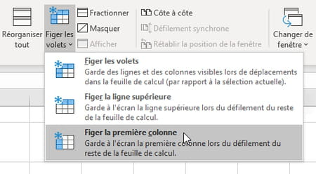
• To freeze more than one column, for example the first two columns A and B : before launching the command Shut downclick at the top, on the column c To select it (you could also just select the cell C1). Now click on the icon Shut downthen below on Shut down. All columns to the left of the column c (so the columns A and B) will now be displayed if you move to the right of the table. In our example, we keep the headers on the screen Years.

• Do not select several columns before launching the command Freeze shutters> freeze shutters. You must only select one, that located to the right of the columns you want to keep visible on the screen.
• Here again, you can cancel the effects by pointing Freeze shutters> release the shutters.

Need to deepen your knowledge about Excel?
Follow our training on CCM Benchmark Institut!

Discover the Excel training on CCM Benchmark Institute

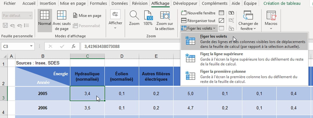
To freeze lines and columns in a spreadsheet, it is essential to select the right cell before launching the command Shut down.

• The option Shut down is in the tab Display. Click on it to unroll the menu presenting its three options. If the first menu option is called Shut downgo to the next step. If her name is Release the shuttersclick on it to cancel the effects and be able to freeze other lines and columns.

• For freeze on lines and columnsselect the cell at the intersection of the lines and columns you want to keep on the screen: by selecting C3 before Shut downTHE lines 1 and 2 and columns A and B will remain visible when you scroll the table on the screen, down or to the right.

• Here again, you can cancel the effects by pointing Freeze shutters> release the shutters.