
When you’re working with a lot of data in your spreadsheet, it can be hard to keep track of everything. It’s one thing to compare one or two rows when dealing with a small subset of data, but when it comes to a dozen rows, things get complicated. And we haven’t even mentioned columns yet. When your spreadsheets get unmanageable, there’s only one solution: freeze rows and columns.
You will also be interested
the freeze Rows and Columns in Excel makes it much easier to navigate your spreadsheet. When done correctly, the chosen panes are locked, which means that those specific rows are always visible, no matter how far you scroll the sheet. Most often you’ll only freeze a few rows or one column, but Excel doesn’t limit the number of rows or columns you can freeze, which can come in handy for larger sheets.
How to freeze a column in Excel?
- Select the row just below the row(s) you want to freeze. If you want to freeze columns, select the cell immediately to the right of the column you want to freeze.
- Go to the View tab and select Freeze Panes > Freeze First Column.
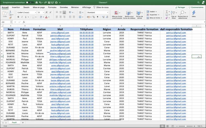
That’s all there is to it. As you can see in our example, the frozen rows remain visible when you scroll down the page. You can tell where the rows have been frozen by the line that separates the frozen rows from the lower rows.
Note that under the Freeze Panes command, you can also choose Freeze Top Row, which will freeze the top row visible (and all others above it) or Freeze First Column, which will keep the leftmost column visible when you scroll horizontally. In addition to allowing you to compare different rows in a long spreadsheet, this feature allows you to keep important information, such as table titles, always visible.
Interested in what you just read?